Application Profiler
Application Profiler is a QNX tool that allows you to view the profiling results generated by instrumented binaries that run on a QNX Neutrino target. The results tell you who called each function as well as how often, how long was spent in each function, and how much CPU time individual lines of codes used. This helps you locate inefficient areas in your code without following its execution line by line.
How to configure Application Profiler
When the launch mode is Profile, the Application Profiler is enabled by default. For other launch modes, you can enable the tool manually through the launch configuration Tools tab (Run, Debug, or Attach modes) or Memory tab (Memory mode). It isn't supported by the Coverage or Check modes.
- Profiling Method
- Profiling Scope
- Options
- Control
Profiling Method
- Functions Instrumentation
- Provides precise function runtimes, based on function entry and exit
timestamps reported by the binary. The binary must be compiled and linked
with the options described in
Enabling function instrumentation
. - Sampling
- Provides runtime estimates based on statistical position sampling driven by
timer interrupts. Your application doesn't need to be recompiled but must
run for a long time for the statistics to be accurate. Also, backtrace
information (call stacks) may not be available. To see call counts, the
binary must be compiled and linked with the option described in
Enabling call count instrumentation
.
Profiling Scope
- Single Application
- Allows you to profile a specific process for an extended period of time, but doesn't provide information about context switches.
- System Wide
- Writes profiling data in kernel events, which are logged to an output file that you can view in the System Profiler tool. When this option is enabled, the IDE initiates a kernel event trace when launching the application. The trace captures kernel activity from all processes on the target. Any kernel event trace should be limited to a few seconds because longer traces produce too much data to be useful.
Options
These options are available only when the Profiling Method is Functions Instrumentation and the Profiling Scope is Single Application.
- Data transfer method
-
- Save on the target, then upload — Saves all profiling data on the target, then uploads the data file to the host when the program finishes. This setting means you can't see results as they come in, but avoids the overhead of sending data over the network while the program runs.
- Upload while running — Sends profiling data to the host while the process runs on the target. This setting lets you see results as they come in, without waiting for the program to finish, but imposes more overhead.
- Path on target for profiler trace
- Sets the location of the profiling results file on the target. You can include the ${random} string, which the IDE replaces with a random number. The IDE can do this replacement in multiple, simultaneous sessions. You can enter either an absolute path that includes the filename or a relative path. If you enter a relative path, the file is written to /tmp.
- Remove on exit
- Removes the profiling results file from the target when the session is complete. If the IDE has substituted a random number for the string ${random} in the filename, the file is permanently removed.
- Use pipe
- Creates a pipe file on the target instead of a regular file. A pipe file stores the collected data using less memory and disk space. To use this option, ensure that the pipe utility is running on the target. For more information, see pipe in the Utilities Reference.
- Profiling Counter
- Specifies which counter the instrumentation code uses to determine the
current time at function entry or exit points.
- Time: Default — Use ClockCycles() for single-core and realtime clock for multi-core (default).
- Time: Clock Cycles — Use
ClockCycles() for multi-core, which is faster
and has better resolution than the realtime clock.
Note:In QNX Neutrino 7.0 or later, we require that the hardware underlying ClockCycles() be synchronized across all processors on an SMP system. This means that threads are no longer required to be bound to the same CPU.
- Time: Clock Monotonic — Use the realtime clock, which reports the monotonic count of elapsed time since the system booted.
- Time: Clock Process — Use the process time clock.
- Time: Clock Thread — Use the thread time clock.
- Memory: Allocated Heap — Use allocated heap memory as a profiling counter (enables memory profiling).
Control
These options are available only when the Profiling Method is Functions Instrumentation, for either a single application or a system wide profiling scope.
- Automatically start profiling
- Specifies whether profiling starts automatically or only after you click Resume Profiling in the Analysis Sessions view. If you uncheck this box, you must define signals for starting and stopping profiling by checking the box just underneath. Otherwise, no profiling results are captured.
- Install start/stop hooks
- Enables the Resume Profiling and
Pause Profiling controls in the Analysis Sessions
view. If your code already uses the default signal numbers that start and
stop profiling, you can specify different values.
- Pause signal number — Specifies the signal number that pauses profiling.
- Resume signal number — Specifies the signal number that starts or resumes profiling.
How Application Profiler results are presented
When you launch an application with the Application Profiler enabled, the IDE switches to the QNX Analysis perspective and opens the Execution Time view, which shows the application's execution time by function. The IDE also creates a session for storing the profiling results, and displays this new session in the Analysis Sessions view.
Analysis Sessions view
This view displays all sessions from analysis tools run on a project within the current workspace. Each session has a header containing the tool icon, binary name, session number, and launch time. Sessions from the Application Profiler, Code Coverage, Memory Analysis, and all Valgrind tools are listed in this view, from the newest (at the top) to the oldest (at the bottom). The session number gets incremented each time a program is run with any of these tools.
For profiling sessions, the icon is a circle with a small clock and checkmark
(![]() ).
Double-clicking the header opens the session (if it's not open)
and displays function information from all components in the
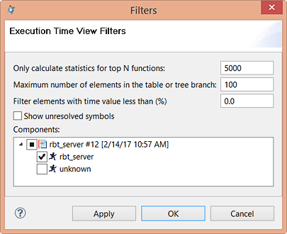
Execution Time view. To filter the results, expand the
header and click the appropriate component. For example, to display results for
functions in your program code but not in any libraries that it uses, click the
application binary.
).
Double-clicking the header opens the session (if it's not open)
and displays function information from all components in the
Execution Time view. To filter the results, expand the
header and click the appropriate component. For example, to display results for
functions in your program code but not in any libraries that it uses, click the
application binary.
When you select an active profiling session, which means the application is still
running, the view toolbar provides
Resume Profiling (![]() ) and
Pause Profiling (
) and
Pause Profiling (![]() ) controls that let you
start and stop profiling. You can specify signals to act as start and stop hooks
for these controls, through the
Control panel.
The Take Snapshot button (
) controls that let you
start and stop profiling. You can specify signals to act as start and stop hooks
for these controls, through the
Control panel.
The Take Snapshot button (![]() ) is also active, and it
allows you to capture the current data without stopping the profiling activity.
You can then compare the snapshot data with the final results or other snapshots.
) is also active, and it
allows you to capture the current data without stopping the profiling activity.
You can then compare the snapshot data with the final results or other snapshots.
Execution Time view
- Name — The name of the function.
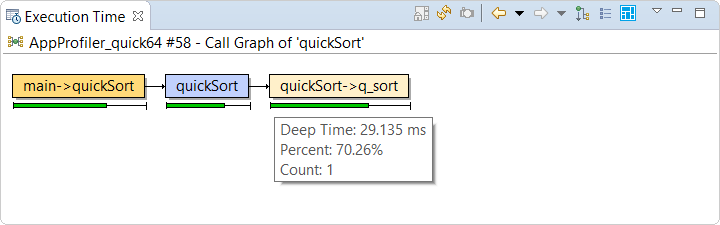
Deep Time — The time it took to execute the function and all of its descendants. This metric is also referred to as Total Function Time. It is the pure realtime interval from when the function started until it ended, which includes its shallow time, the sum of its children's deep times, and all time in which the thread wasn't running while blocked inside of it. If the function was called more than once, this column contains the sum of all runtimes when it was called from a particular stack frame or parent function.
Inside each column entry, on the left, a green bar and percentage value indicate the relative execution time. On the right, another value indicates the absolute execution time.
For Sampling mode, this column isn't used.
Shallow Time — For Function Instrumentation mode, this column is the deep time minus the sum of its children's runtimes. It roughly represents the time spent in this function only. However, it also includes the time for kernel and instrumented library calls and for profiling the code.
For Sampling mode, it's an estimated time, calculated by multiplying an interval time by the count of all samples from this function.
The column entries have a green bar overlaid with a percentage value (on the left) and another numeric value (on the right). These items provide similar information as in the Deep Time column.
- Count — The number of times the function was called.
- Location — The location of the function in the code.
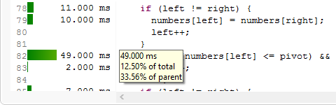
- Percent — The percentage of Deep Time compared to the Total Time (or compared to the Root Node Time).
- Average — The average time spent in the function.
- Max — The maximum time spent in the function.
- Min — The minimum time spent in the function.
- Time Stamp — A timestamp indicating the last time the function was called, if present.
- Binary — The binary filename.
Call sequence information.
- Disable Automatic Refresh (
 ) —
Pause the data display in its current state until you unlock it.
) —
Pause the data display in its current state until you unlock it. - Refresh (
 ) — Refresh the data display.
- Take Snapshot and Watch Difference (
 ) — Create a profiling
session that is a snapshot of the current data. Later, you can
compare the results of two sessions to see the
effects of any changes you made between execution runs.
) — Create a profiling
session that is a snapshot of the current data. Later, you can
compare the results of two sessions to see the
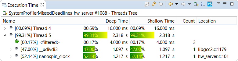
effects of any changes you made between execution runs. - Show Threads Tree (
 )
— Display a graphical representation of the threads and calling
functions within your application. This display helps you see exactly
where the application spends its time and which functions are most used.
You can examine the details down to the lowest function calls.
)
— Display a graphical representation of the threads and calling
functions within your application. This display helps you see exactly
where the application spends its time and which functions are most used.
You can examine the details down to the lowest function calls.
Note:Information about individual threads is not available for postmortem profiling. Instead, only one thread (with all time assigned to it) is displayed. - Show Table (
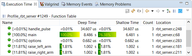
 ) — Display a list of functions
within your application. This display helps you identify which functions
take the longest to complete. In Functions Instrumentation mode, calls to C
library functions such as printf() are not displayed.
) — Display a list of functions
within your application. This display helps you identify which functions
take the longest to complete. In Functions Instrumentation mode, calls to C
library functions such as printf() are not displayed.
Annotated source
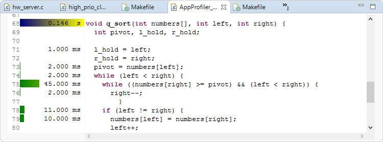
- Blue-Yellow
- For the first line of a function, a blue-yellow bar shows its total runtime. This includes the function's shallow time, the sum of its children's deep times, and all time in which the thread wasn't running while blocked inside of it.
- Green
- For a line of code, a green bar shows the amount of time for the inline sampling or call-pair data. The lengths of the green bars within a function add up to the length of the blue-yellow bar on its first line.
Call sequence information
- Show Calls
- List all functions called by the selected function. The resulting list lets you examine specific call chains to find which ones have the greatest performance impact. You can expand the entries of descendant functions to see how execution time is distributed among them.
- Note:For this and other options, you can use the Go Back (
 ) and
Go Forward
(
) and
Go Forward
( ) toolbar buttons to move
between the menu action results and original profiling results.
) toolbar buttons to move
between the menu action results and original profiling results. - Show Reverse Calls
- List all callers of the selected function. The resulting list shows the execution times for all calling functions. The same columns are shown, and you can right-click again and choose this same option or Show Calls, to navigate up or down a particular call stack.
- Show Call Graph
- Display a graph of how the functions are called within the program.
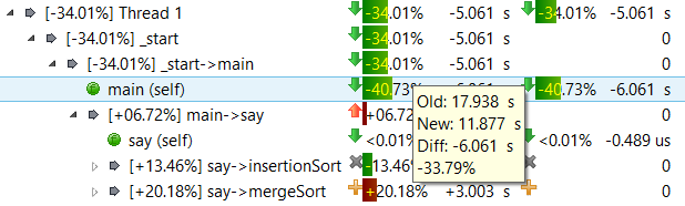
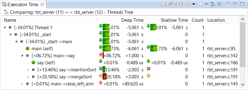
Interpreting differences in session results
You can compare the results of two profiling sessions to see the effect of changes you made to an application. The comparison feature calculates and displays the differences in function runtimes and other metrics between the sessions, in the Execution Time view.
 —
Function runtime has decreased.
—
Function runtime has decreased. —
Function runtime has increased.
—
Function runtime has increased. —
Function was called in first session only.
—
Function was called in first session only. —
Function was called in second session only.
—
Function was called in second session only.