![[Previous]](prev.gif) |
![[Contents]](contents.gif) |
![[Index]](keyword_index.gif) |
![[Next]](next.gif) |
|
|
|
|
 |
This version of this document is no longer maintained. For the latest documentation, see http://www.qnx.com/developers/docs. |
You can select a topic from this diagram:
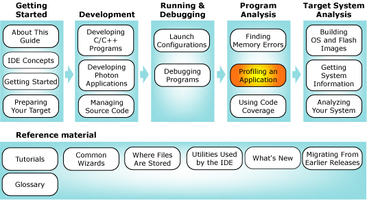
This chapter shows you how to use the Application Profiler tool.
In this chapter:
The QNX Application Profiler perspective lets you examine the overall performance of programs, no matter how large or complex, without following the source one line at a time. Where a debugger helps you find errors in your code, the QNX Application Profiler helps you pinpoint inefficient areas of your code that could run more efficiently.
The QNX Application Profiler perspective.
By default, the Application Profiler perspective includes these main views:
The QNX Application Profiler lets you perform:
Sampling doesn't require instrumentation, and has low overhead, but your application needs to run for a long time for you to get sound data.
Sampling and Calls Countrequires a compiler and linker flag, and has more overhead.
Function Instrumentation requires a compiler flag and linker flag, and even more overhead.
The QNX Application Profiler takes "snapshots" of your program's execution position every millisecond and records the current address being executed. By sampling the execution position at regular intervals, the profiling tool quickly builds a summary of where the system is spending its time in your code.
With statistical sample profiling, you don't need to use instrumentation, change your code, or to perform any special compilation. The profiling tool profiles your programs unobtrusively, so that it doesn't bias the information it's collecting.
 |
The results are subject to statistical inaccuracy because the profiling tool works by sampling. Therefore, the longer a program runs, the more accurate the results. |
This method provides you with precise function run time information for your project. It performs better on one thread, because with many threads, the overhead of such measurement can change the application's behavior.
To enable instrumentation, compile each source file with the option -finstrument-functions. This gcc option instructs the compiler to generate a call to the profiling function just after the entrance to, and just before the exit from every application function, which permits the collection of profiling information. Profiling functions are defined in the libprofilingS.a library; to access these, link the binary or library with the -lprofilingS option.
|
For an application that intends to use an instrumented library as a DLL (i.e. using a dlopen() call), compile the library with the -Wl,E option. |
This type of profiling is a combination of sampling mode and Call Count instrumentation data, and it provides per line statistical coverage (as well as a call graph at the same time), with relatively small overhead.
To instrument a binary or library in this mode, use the -p option for both compiling and linking. The -p option for the compiler prepares the binary for profiling (the compiler will then insert code before each function to gather call information); however, it won't cause the profiling versions of the libraries to be linked in. To link in the profiling versions from the libc library, use the -p option for the linker.
If you compile and link with either the -pg or -p option, when the executable program runs, either gprof or prof monitors the program and produces a report file called gmon.out. The gprof utility can't report information about program calls to routines from a precompiled library (such as libc) that weren't compiled with the -pg option. Consequently, the resulting profiling information won't include data about calls made to those routines (for example printf()).
If most of the execution time occurs in various library routines, then this fact will likely reduce the value of the profiling results, since there is no indication in the results of where the call was made. In this case, you can use Function Instrumentation profiling, which causes this additional time to be charged to the higher-level routine that called the library function.
The IDE lets you examine profiling information from an output file produced by an instrumented application (i.e. gmon.out). The tool provides you with all of the information collected at runtime, but in a graphical format.
Postmortem profiling supports data generated by gprof (gmon.out), the QNX profiler library (.ptrace), and the trace logger (.kev).
For more information about the gprof utility, go to www.gnu.org; for qcc, see the Utilities Reference.
Whether you plan to do profiling in real time or postmortem, you'll need to build your programs with profiling enabled before starting a profiling session (for Instrumented profiling).
This section includes these topics:
|
If you already have a gmon.out, .kev, or .ptrace file, you're ready to start a postmortem profiling session. |
Although you can profile any program, you'll get the most useful results by profiling executables built for debugging and profiling. The debug information lets the IDE correlate executable code and individual lines of source; the profiling information reports call graph data or precise function time measurements.
|
Sampling and Call Count profiling is handled by functions in libc; Function Instrumentation profiling is handled by functions in libprofilingS.a; occasionally check our website for any updates to these libraries. |
This table shows the Application Profiling features supported with the various profiling modes:
| Feature | Sampling | Sampling and Call Count | Function-Instrumentation |
|---|---|---|---|
| Own Function Time | Yes | Yes | Yes |
| Thread Time | Yes | Yes | Yes |
| Start/Stop Profiling | Yes | Yes | Yes |
| Source Location (if compiled with debug) | Yes | Yes | Yes |
| Line level editor annotations | Yes | Yes | No |
| Function calls editor annotations | No | No | Yes |
| Thread tree mode | Yes | Yes | Yes |
| Table mode | Yes | Yes | Yes |
| Call graph mode | No | Yes | Yes |
| Who calls/Who called | No | Yes | Yes |
| Calls Count | No | Yes | Yes |
| No recompile | Yes | No | No |
| Function backtrace | No | No | Yes |
| Deep Function time (own + descendants) | No | No | Yes |
| Timed stack tree | No | No | Yes |
| Max/Min Time | No | No | Yes |
For an existing project, when you build your project to profile an application to capture performance information, profiling can provide you with decision-making capabilities to help discover functions that consume the most CPU time. However, to instrument your code, you'll need to change the existing configuration options so that you can build your project with profiling enabled. The IDE will then insert code before each function to gather call information (Call Count instrumentation) or just after the function enters, and just before the function exits (Function Instrumentation).
To configure profiling for the selected project, depending on your type of project, do one of the following:
|
For example, your Makefile might have a line like this:
CFLAGS=-p CXXFLAGS=-p LDFLAGS=-p |
|
The QNX Application Profiler uses the information in the debuggable executables to correlate lines of code in your executable and the source code. To maximize the information you get while profiling, use executables with debug information for both running and debugging. |
To run and profile a process, with qconn on the target:
|
Debug mode isn't recommend for running Function Instrumentation mode, because it can skew the profiling data results. |
|
To run in Sampling mode, select Sampling and Call Count Instrumentation; to run in Sampling and Call Count mode, select Sampling and Call Count Instrumentation; to run in Function Instrumentation mode, select Function Instrumentation and Single Application. For descriptions about these options, see "Application Profiler tab." |
The IDE starts your program and begins to profile it.
To produce full profiling information with function timing data, you need to run the application as root; this is required when running through qconn.
If you run the application as a normal user, the Application Profiler tool can generate only call-chain information.
You have to specify the Shared library path in two locations: use the Uploads tab in the launch configuration if libraries have to be uploaded every time an application runs, and use the Shared Libraries tab on the Tools tab to specify the host location of libraries so that the IDE can read their debug symbols to show their symbol information.
Since the dynamic library isn't included with the IDE, there is an issue caused by the static linkage of the profiling library. To solve this problem, you'll need to do the following:
Make sure that the text box for Linker options includes the -Wl,-E options.
You can run a process on the target (without the IDE) and collect the profiling information while it's running. In order to collect profiling information, you have to modify the way you normally launch your application by adding environment variables:
|
If you're launching using the IDE, you can specify the environment variables on the Environment tab in the launch configuration. |
To profile a process that's already running on your target:
|
When you profile a running process, you can't use the Console view in the IDE to interact with this process. If your running process requires user input through the Console view, use a shell to interact with the process. |
For descriptions about the options, see "Application Profiler tab."
The IDE doesn't know the location of your shared library paths, so you must specify the directory containing any libraries that you wish to profile. For a list of the library paths that are automatically included in the search path, see the appendix Where Files Are Stored.
Postmortem profiling lets you profile your application (the data generated by the profiling process) at a later time. The IDE lets you profile your program after it terminates, using the traditional gmon.out file; however, postmortem profiling doesn't provide as much information as profiling a running process because:
Profiling a gmon.out file involves these basic steps:
To gather profiling information in a gmon.out file, you need to specify the PROFDIR environment variable before launching your application.
If you're launching from the command line, type the following:
PROFDIR=/tmp ./appname
To launch from IDE:
|
You must have the QNX Application Profiler tool disabled in your launch configuration. |
|
This path must be a valid location on the target machine; otherwise, you'll receive a warning message indicating that the IDE was unable to open the gmon.out file for output. |
You can import .gmon, .kev, .ptrace, or .xml data files using the Import action from the session view, or using the Import wizard:
To create a .ptrace file, run your application with the option QPROF_FILE=/tmp/app.ptrace. For example, to launch from the command line, type:
QPROF_FILE=/tmp/app.ptrace ./appname
To launch from the IDE:
The descriptions for the launch options for the Application Profiler tab are:
The Profiler Sessions view () lets you control multiple profiling sessions simultaneously. You can:
The Profiler Sessions view.
From the Debug tab, you can see more detail about the session:
The Debug tab for profile sessions.
The Profiler Sessions view shows the following as a hierarchical tree for each profiling session:
| Type | Description |
|---|---|
| Session ID | A consecutive identifier assigned to each profiler session. |
| Session Name | Launch instance name (i.e. ApplicationProfiling). |
| Session State | The current state of the session (open, closed) |
| Session Timestamp | The date and time the session was created. |
The icons that appear in the Profiler Sessions view are:
| Name | Icon |
|---|---|
| Running Process | |
| Executable | |
| Shared libraries | |
| DLLs | |
| Unknown |
|
A node named Unknown refers to a container for code that doesn't belong to any binary or library. Usually, this type refers to kernel code mapped to process virtual memory. For Sampling and Call Count profiling, not all shared libraries or the binary appear in the tree view. The view can include only those libraries and binaries that were instrumented with Call Count instrumentation, or those that have corresponding samples during the execution. If the application runs for a short period of time (less than ten seconds), a library might not even have a single probe. For Function Instrumentation, profiling only an instrumented binary and libraries would display in the tree view. System libraries, such as libc, would never appear in the view. |
To terminate an application running on a target:
|
To clear old launch listings from this view, click the
Remove All Terminated Launches button ( |
To disconnect from an application running on a target:
|
To clear old launch listings from this view, click the Remove All Terminated Launches button ( |
Other views within the QNX Application Profiler perspective show the profiling information for each item you select in the Profiler Sessions view.
| This view: | Shows: |
|---|---|
| Profiler Sessions | Application Profiler sessions |
| Execution Time | Function Instrumentation or Call Count |
| Debug | Target debugging in a Debug tree hierarchy view and the Application Profiler Debug view |
| Annotated source editor | The amount of time your program spends on each line of code and in each function |
| Properties | Session or item properties |
After gathering the profiling data, you can change to the Application Profiler perspective, and begin to analyze the data. In the Execution Time view, after profiling a project, the results show as precise function execution time, and a runtime call graph for Function Instrumentation. The results show the time for each function when Call Count profiling is enabled.
The Profiler Sessions view contains the sessions for the profiler instances. The other views within the QNX Application Profiler perspective are updated to show the profiling information for each item that you select from this Profiler Sessions view.
| Icon | Name | Go to |
|---|---|---|
| Resume Profiling | Pausing and resuming a profiling session | |
| Pause Profiling | Pausing and resuming a profiling session | |
| Take Snapshot of the running session | Taking a snapshot of a profile session | |
| Create a Sample Session | Creating a sample profile session | |
| Export Application Profiler Session | Exporting a profiler session | |
| Import Application Profiler Session | Creating a profiler session by importing profiler data |
Occasionally, having too much data is the same as having no data at all. You can take control of when to enable profiling during the execution of an application using the Pause and Resume icons in the toolbar.
This feature lets you freeze the current state of the Application Profiler data while the actual session data keeps changing. The snapshot data remains frozen and can later be compared with the final results, or other snapshots of the same session. However, in the Execution Time view, this action also automatically switches to a comparison mode to dynamically show the updated difference between the current state and the snapshot.
A sample profile session will provide you with sample data to quickly evaluate features of the application profiler.
In the IDE, you can export your profile data information from the Profile Sessions view. When exporting your profiling analysis information, the IDE lets you export the results in the format you specified during export.
To export a profiler session:
Later, you can import data (see Creating a profiler session by importing profiler data), or you can choose to import other session data into System Profiler to review the results (see Using the results from Function Instrumentation mode in the System Profiler).
The Debug view shows the target debugging information in a tree hierarchy.
The Debug view.
The number displayed after a thread label is a reference counter, not a thread identification number (TID).
The IDE shows stack frames as child elements, and it shows the reason for the suspension beside the thread, (such as the end of the stepping range, a breakpoint was encountered, or a signal was received). When a program exits, the IDE also shows the exit code.
This view provides you with valuable decision-making capabilities in that it helps you identify those functions that clearly consume the most CPU time, making them candidates for optimization. This type of instrumentation is the most effective way of optimizing bottlenecks in a single application. This data-collection technique lets you gather precise information about the duration of time that the processor spends in each function, and provides stack trace and Call Count information at the same time.
The Execution Time view in the Application Profiler perspective.
Using a call tree, you can see exactly where the application spends its time, and which functions are used in the process.
By default, the selected preferences provide you with the basic columns containing valuable profiling data; however, you can specify additional columns and display settings (see "Setting preferences"), if desired.
The Execution time view supports the following tree views and graph:
The following table describes the meanings for time columns for all data source combinations with visual modes:
| Mode | Node | Time | Own Time | Count | Average | Max (Min) |
|---|---|---|---|---|---|---|
| Sampling and/or Call Count | Function (All) | Same as Own Time, invisible | The sum of all problems for a given function | The sum of Count for all Call Samples where given function is "to" | Own Time / Count, or Own Time if count is 0 | N/A |
| Sampling and/or Call Count | Addressable (All) | Same as Own Time, invisible | The sum of all problems for a given address, or 0 if no problems for a given address (but exists in the Call Counts tree) | The sum of Count for all Call Samples where given function is "to" | Own Time / Count, or Own Time if count is 0 | N/A |
| Sampling and/or Call Count | Line Probe (Call Tree mode) | Same as Own Time, invisible | The sum of all problems for a given address | 0 | Same as Own | N/A |
| Sampling and/or Call Count | Call Pair (Call Tree mode, Reverse Call Tree mode) | N/A | N/A | The sum of Call Counts a for given pair | N/A | N/A |
| Sampling and/or Call Count, Function Instr. | Group Node (Reverse Call Tree Mode, Table Mode) | Same as Own Time | The sum of Own Time for the children | The sum of Count for the children | Time / Count | Max (Min) of children |
| Function Instr. | Function (All) | The sum of the Total Function Time for each occurrence of this function in a timed call tree, excluding inner recursive frames | The sum of the Own Function Time for all occurrences of this function in a call tree. The Own Function Time for the call tree is the Total Function Time minus the sum of the Total Function Time for all descendants. | The sum of all counts to this function in the call tree | (Time + Rec. Time) / Count | The Max (Min) of the Total Function Time between all occurrences |
| Function Instr. | Thread (Call Tree mode) | The sum of the total for entry functions (only one entry, but there might be some unattached calls) | Same as Total | 1 | N/A | N/A |
| Function Instr. | Call Pair (Call Tree mode) | The sum of the Total Function Time for all occurrences of this call pair for a given parent backtrace | N/A | Call Count of this call pair for a given parent backtrace | Time / Count | Max (Min) of this call pair's Total Time for a given parent backtrace |
| Function Instr. | Self (Call Tree mode) | Same as Own | The parent Total minus the sum of the Total for the siblings | Count of a parent | Own Time / Count | Max (Min) of this call pair's Own Time for a given parent backtrace |
| Function Instr. | Recursive Call Pair (Reverse Call Tree mode) | N/A | N/A | The sum of Call Counts for a given pair | N/A | N/A |
| Function Instr. | Call Pair, Thread, Process (Reverse Call Tree mode) | The sum of Total Call Pair time for the Root function for a given stackframe (the child in this tree represents the parent in the call stack) | N/A | The sum of Call Counts for the Root function for a given stackframe | Time / Count | N/A |
| Icon | Name | Description |
|---|---|---|
| Scroll Lock | Pauses the current view of the data to show the results to you in a frozen state until you unlock the window. | |
| Refresh | Updates the current view to show the most recent profiling information. | |
| Take Snapshot and Watch Difference | Take Snapshot and Watch Difference | |
| Go Back | Moves up one level in the tree view hierarchy. | |
| Go Forward | Moves down one level in the Tree view hierarchy. | |
| Show Threads Tree | Show Threads Tree | |
| Show Table | Show Table mode | |
| Menu | Shows the menu of options for this window. |
Use the Take Snapshot and Watch Difference icon to create another profiler session that's a snapshot of your program. Later, you can use the Compare feature to compare the profile session data, and then continue to monitor the results as your application runs in another pane.
The Show Threads Tree option lets you show a graphical representation of the threads and calling functions within your application. You can drill down to see the detail of the lowest function calls.
The Show Threads Tree view.
You can use this information to:
This mode shows a list of functions from the applications in your project.
|
In Function Instrumentation mode, it doesn't show calls to functions, such as printf(), in the C library. |
![]()
A list of functions for the selected profile is displayed in the Execution Time view.
The Show Table Mode view.
From this table, select a function a right-click to Show Calls, Show Reverse Calls, Show Call Graphs, or Show Source.
The Call Tree mode shows you a list of all of the functions called by the selected function. This call tree view lets you drill into specific call traces to analyze which ones have the greatest performance impact. You can set the starting point of the call tree view by drilling down from a thread entry function to see how the actual time is distributed for each of its function descendants.
Time columns contain the following features, which you can customize using the Preferences menu option:
Additional columns:
A reverse call tree shows you what is calling a specific function, and how its time was distributed for each of those callers. You can use a reverse call tree to either drill up or down the stack to view the callers and their contribution time, until you encounter a thread entry function.
A call graph shows a visual representation of how the functions are called within the project.
A simple example of a call graph.
This call graph shows a pictorial representation of the function calls. The selected function appears in the middle, in blue. On the left, in orange, are all of the functions that called this function. On the right, also in orange, are all of the functions that this function called.
|
You can show the call graph only for functions that were compiled with profiling enabled. If you position your cursor over a function in the graph, you will see Deep Time, Percent, and Count information for that function, if any. For descriptions about these fields, see Field descriptions. |
Occasionally, you'll want to view the source code for a particular function that might require further investigation. You can easily jump to the source code and compare the profiling results against the actual code to determine if the data is acceptable, or if it's a candidate for further optimization.
An easy to use context navigation menu is available for each node of the tree, table, or call graph. The options available from the context menu are:
The Execution Time view includes the following features:
You can create a second Execution Time view to see data side-by-side in another window using the menu option Duplicate View. The new view is disconnected from Profiler Sessions view; however, it maintains its own history. You can use this feature to observe a "snapshot" of your program, and then continue to monitor the results as your application runs in another pane.
The Execution Time view keeps track and maintains a record of where have been. You can use the Go Back and Go Forward icons from the toolbar, or select a particular entry in the navigation history. You can set the navigation history size in the preferences for the view.
The grouping feature helps for the organization of large function tables, and for improved navigation and analysis. This is the most efficient method to observe aggregated time results for each software component (binary or file).
Menu options for grouping.
You can use the Execution Time View Preference Page to customize the number of columns you want to have in the view, their order, and the format of the data they show in the view.
Setting user preferences.
For example, you might want to select more columns to add more detail information to your view:
Additional columns selected for the view.
At any time, if you want to see the table or tree data in textual format, use your development host's method of copying to obtain the text version of the visible data, which will be copied to your clipboard.
When grouping doesn't help reduce the amount of profiling data from the results, you can use filters to remove some rows from the table. Component filtering lets you see only those records related to the specified component, or you can use Data filtering to filter based on timing values.
When filtering is applied, the "<filtered>" element remains in the view as a remainder of the filtered elements, and the total number of these elements is visible in the Count column.
The Filtering dialog.
You can perform a text search on the data results from the profile. The Find feature includes a Find bar at the bottom of the Execution Time view. The view automatically expands and highlights the nodes in the tree when the search locates results matching the search criteria.
The annotated source editor lets you see the amount of time your program spends on each line of code and in each function.
To open the editor:
|
You may receive incorrect profiling information if you change your source after compiling because the annotated source editor relies on the line information provided by the debuggable version of your code. |
The annotated source editor shows a solid or graduated color bar graph on the left side, as well as providing a Tooltip with information about the total number of milliseconds for the function, the total percentage of time in this function, and for children, the percentage of time in the function as it relates to the parent.
The length of the bar represents the percentage. On the first line of the function declaration, that bar provides the total for all time spent in the function. The totals include:
The colors on the bars represent:
The QNX annotated source editor.
If you want to profile an application, you can do the following:
When you profile a project, you can choose Function Instrumentation to obtain detailed information about the functions within your application. Each function entry and exit is instrumented with a call. The purpose of this is to record the entry and exit time of each function and call sequence.
The profiling options available to you are:
Sampling mode provides you with profiling information for your project at a specific time interval (the Application Profiler takes samples from processes at given rate). The information is recorded into a sample that you can use for comparison purposes.
|
When you use sampling mode to obtain only data, you'll notice the following:
|
To prepare your binary for Call Count instrumentation:
To build a C/C++ project for profiling, compile and link using the -p option. For example, your Makefile might have a line like this:
CFLAGS=-p CXXFLAGS=-p LDFLAGS=-p
Now, your application is launched, as well as the Application Profiler tool. The Application Profiler perspective opens and the Execution Time view shows data from the current session; the view is automatically refreshed.
To customize your Execution Time view if you're running in this mode:
This method lets you obtain precise function information at runtime. It performs best for one thread because when there is more than one thread, the overhead measurement from multiple threads can change the application's behavior.
To compile an application with Function Instrumentation:
|
If the process doesn't finish, you'll have to terminate it manually. Instead of terminating the process, you can terminate the Application Profiler service in the Debug view; the IDE will download the current state of the data. The Application Profiler isn't optimized for data transfer; each second of application running time can generate up to 2 MB of data. |
|
If the binary wasn't compiled on the same host, you'll need to edit the Source Path tab to add the source search path or mapping between the compiled code location and the location of the source on the host machine. |
The IDE creates a profiler session and automatically selects it.
By using the data from the Function Instrumentation mode in System Profiler, you can:
By default, you won't see function names, only addresses; however, you can manually add binary information by doing the following:
Application Profiler data in the System Profiler timeline.
|
If you're missing function names in the System Profiler Timeline view, you may want to consider adding this information by instrumenting your binaries with the Function Instrumentation library, and running in Kernel Events mode. For additional information, see "Using Function Instrumentation mode for a single application." |
To launch from the command line:
QPROF_KERNEL_TRACE=1
Set this environment variable for each process, or export it for all processes; it won't affect uninstrumented binaries.
|
You can use tracelogger to capture events generated by programs compiled with Function Instrumentation. |
To profile a process:
When you create an Application Profiler session, you can profile an application to capture performance information after you've created your launch configuration.
Before you start:
To profile in this scenario, follow these steps:
Now, the Application Profiler session is ready for you to use.
You can create a profiler session by importing .gmon, .kev, or .ptrace files using the Import action from the Profiler Sessions view.
Before you start, you must:
To profile in this scenario, follow these steps:
The IDE creates a new Application Profiler session and populates it with the imported data, as well as the Execution Time view. Now, your Application Profiler session is ready for inspection.
For this particular situation for example, you might have a single-threaded application that performs badly for a specific test case, and you want to understand the reason(s) why, and try to attempt to optimize it, if possible.
Before you start:
Before you start:
To profile the application, follow these steps:
The IDE changes to the Application Profiling perspective, populates the session view, and shows the Execution Time view, which dynamically changes.
The active page shows the Tree containing the list of functions being called.
Now, you can investigate why the certain functions consume the CPU time.
Now, you might notice that this function is called from other places as well; however, you need to investigate its total contributions versus the amount of CPU it consumes.
Next, you can confirm your results by running another profiling session, and then using the Compare feature to compare the results.
The IDE opens a view where you can see the total time compared to the other session time with the percentage of improvements (a green arrow pointing downward).
|
There's no need to change your compile options. |
You can profile an application to capture performance information for an existing project.
Before you start:
The process must be running on the target with profiling enabled.
To profile a process from an existing QNX C/C++ project that's already running on your target:
You can change the configuration options to profile an application to capture performance information whereby profiling is done by code linked into the process, and after the process exits normally (without error). Data, which is the function information (such as call counts, callers, and statistics), is written to a file that you can then load into the IDE.
To configure postmortem profiling:
Profiling information is written to a file in the location you specify with the PROFDIR environment variable. If you don't set PROFDIR, the information is written to a file called gmon.out in the directory the process was run from.
Now, you can begin to analyze the profiler data.
When it's not possible to run an application from the IDE, but it's possible to re-compile application, run it on a target and transfer results back to host machine, you can use the results of postmortem profiling to transfer the results using the Import wizard.
To profile the application, follow these steps:
Next, create a profiler session by importing profiler data. Ensure that you compile the binary with instrumentation enabled.
![]()
The Application Profiler Import wizard opens.
The IDE creates a new Application Profiler session and populates it with the imported data, as well as populating the Execution Time view with data.
Application Profiling Session is ready to use.
To run an instrumented binary with profiling from the command prompt:
QPROF_START=1
QPROF_FILE=/tmp/myapp.ptrace
LD_LIBRARY_PATH=.../profiling_lib:$LD_LIBRARY_PATH
	QPROF_START=1 QPROF_FILE=/tmp/myapp.ptrace \
	LD_LIBRARY_PATH=.../profiling_lib:$LD_LIBRARY_PATH  ./myapp
A snapshot of a profiling session provides you with a record of the current state of the session data from the moment you select the capture option. You can then use the snapshot to look for differences in CPU time between the time of the snapshot and the running time of the profiling session that followed.
To take a snapshot of a profiling session, follow these steps:
The snapshot capture freezes the current state of the Application Profiler data; meanwhile the actual profile session data keeps changing. Now, you can begin to analyze the profiler data to compare the snapshot data against the changing data.
When you complete optimizing, it's useful to see what progress you've made. The comparison mode lets you easily see the difference between two profile sessions. You can continue to view data as a Call Tree or a Table, but instead of absolute time values, you see time differences.
For example, you can compare two profiles to evaluate results before and after function optimization. In Compare mode, each column shows the change in values compared to the other session. Time and Count columns show the new value minus the old value. If there's no new value match for an item, its old value is used. If no old value match exists, the item will have a "+" indicator beside the new value.
Comparing two profiler sessions.
In this case, you must have at least two Application Profiler sessions to compare.
To profile in this case, follow these steps:
View the changes based on the results of the Comparison mode.
The Execution Time view shows the difference between two selected sessions, and you can observe these differences by:
|
In the Profiler Sessions view, you can use the Take Snapshot feature to freeze the current state of the Application Profiler data while the actual session data keeps changing. The snapshot data remains frozen and can later be compared with the final results, or other snapshots of the same session. In the Execution Time view, this action also automatically switches to view a Comparison mode to dynamically show the updated difference between the current state and the snapshot. |
|
|
|
|